How to format dates in Google Sheets

You can change the format of dates in Google Sheets, autofill dates or sort rows by date. Being able to do so can save you a lot of work and give you a better overview of your document.

Why is it important to have a uniform date format in Google Sheets?

In some spreadsheet applications, the method for inputting dates isn’t ideal. Auto-correction or imprecise formatting can lead to documents that are inconsistent and cluttered. There are also a number of different date formats, which can vary by language or specific use case. Learning how to handle dates in your spreadsheet can save you considerable time and help you to create more organised documents. Below, you’ll find everything you need to know about managing dates in Google Sheets.

What is the DATE function in Google Sheets?

Just like Microsoft Excel’s DATE function, Google Sheets also has a function called DATE. This is used to automatically convert entries that contain a year, month and day into an actual date. The syntax of the function looks like this:

DATE(year, month, day)

There are a few things that you should keep in mind when using this function. First, the date can only be output if all entries are made up of numbers. If a character string is entered, Google Sheets will display an error message. However, if you enter incorrect values (e.g. a month value over 12 or a day value over 31), the output is automatically recalculated with the excess values taken into account. For example, the input DATE(2024,1,33) becomes 02.02.2024 since January only has 31 days. The function shortens decimal values and issues an error message for values above 10000 and below 0.

You can find an overview of the most important keyboard shortcuts for Google Sheets in our Digital Guide.

How to insert dates in Google Sheets

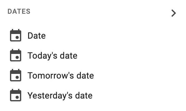
Another quick method for inserting dates in Google Sheets is to use the [@] key. To do this, follow the steps below:

1. Click the field where you want to insert the date.
2. Press the [@] key.
3. Next to files or other contacts; you’ll find the option Date.
4. You now have various options to choose from. If you click on Date, the calendar will open, and you can select any date. Alternatively, you can choose Today’s date, Tomorrow’s date or Yesterday’s date in Google Sheets.

How to easily format dates in Google Sheets

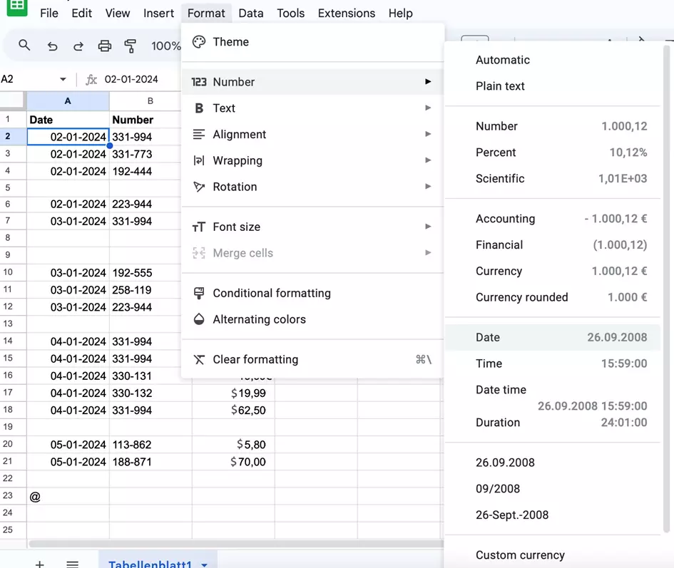
When you open a new spreadsheet document, you can insert a date in any format. This includes formats such as ‘01.01.2024’, ‘1.1.2024’, ‘1/1/2024’ or ‘1-1-2024’. By default, the program will accept these inputs as they are, which might cause inconsistencies in the document. You can use the following method to format the basic numerical values:

1. Click on the field that you want to edit, or alternatively, select several fields.
2. You’ll find the Format option in the tab along the top. Select this.
3. Second on the list, you’ll find the option Number. Click on it.
4. Select Date. All selected numerical values will now be converted to the standard ‘Day.month.year’ format.

You also have the option of determining the format yourself. Here’s how to choose the format yourself:

1. Select the relevant field or fields again.
2. Click on Format and then on Number.
3. Near the bottom of the list of options, you’ll find the option Custom date and time. Select this option.
4. You’ll now be presented with a list of different date and time formats. For example, you can include the day of the week, have the name of the month written out or display numerical values under 10 in single digits. Select the format you want and then click Apply. The dates you selected will now be converted into this format.

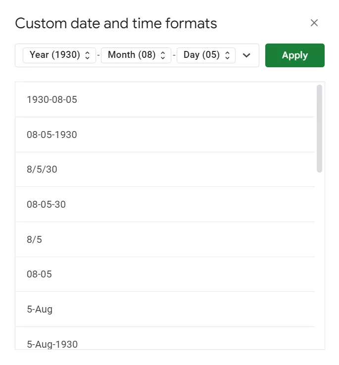
It’s possible to customise the format even more. You can start by choosing the format you want to use and make adjustments using the arrows next to each element. For example, you can decide to drop the first zero from the day, display the month’s name fully or show the year with just two digits. If you prefer to use dashes instead of dots to separate items, you can specify this in the settings. Once you are satisfied with the adjustments, click Apply.

How to format consecutive dates in Google Sheets

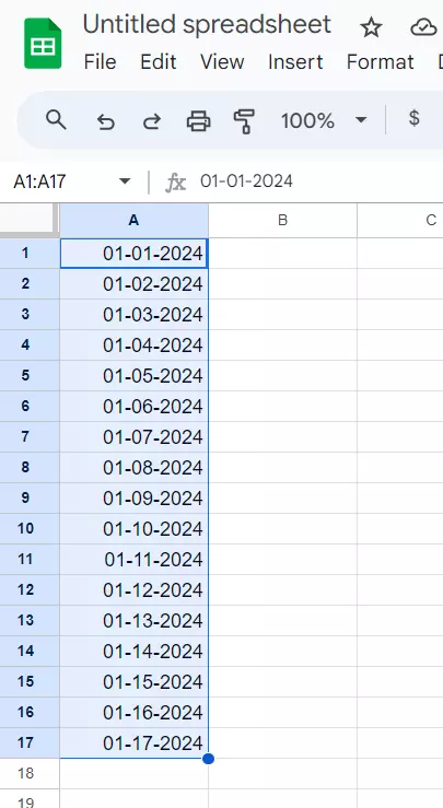
If you want to add consecutive dates in a Google spreadsheet, you don’t have to enter each one manually. Instead, simply follow the steps below:

1. Click inside the field where you want to start your list.
2. Enter the first date manually in your preferred format.
3. Move the mouse pointer to the bottom right-hand corner of the field. A small plus sign will appear. Click on it.
4. Hold down the mouse pointer and drag the cursor downwards.
5. Release the mouse pointer. The program will now automatically complete the individual days up to the field you have selected.

How to sort Google Sheets by date

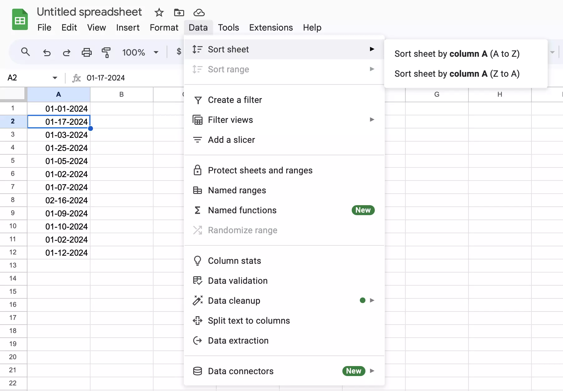
There is also a practical trick for sorting your Google spreadsheet by date. This is useful if you have numerous entries with dates that aren’t in sequential order. You can write down the items in any order and then simply follow these steps here:

1. Click on the column with the dates.
2. Now select the Data tab from the menu at the top of the screen.
3. Click on Sort sheet. You can choose whether the entries should be sorted in descending or ascending order.