Excel CONCATENATE function explained

Microsoft’s spreadsheet software lets you perform difficult calculations and interesting analyses. But there are times when you may want to combine multiple elements in a single result. The Excel CONCATENATE function lets you do just that. We’ll explain how it works.

In Excel, the results of a calculation are usually shown in the corresponding cell. You can nest multiple functions to perform complex calculations and obtain a single result. But sometimes you may want to combine multiple elements in a single cell. The CONCATENATE function lets you do just that. For example, assume you’re given an Excel spreadsheet with months of the year in one column and the average temperature in another (column 1: Jan, Feb, March; column 2: 10, 12, 20). Rather than display two separate columns, you can merge these results into a single cell per row (e.g. “Jan 10”, “Feb 12”, “March 20”. Excel CONCATENATE lets you combine text, numbers and cell references with one another. You can even integrate other functions into the formula, eliminating the need for auxiliary cells in some cases.

In principle, CONCATENATE can be used in two different ways in Excel: as a function or in the form of an operator. The function has at least one argument, but can link up to 255 entries with one another.

Within the function, Excel refers to the parameters as “text” because the formula is intended to combine multiple elements to form a string of text. However, as stated above, you can combine different forms:

• Text: In Excel, you insert text between quotation marks. That tells the programme how it is to process the information.
• Numbers: Numbers can be inserted with or without quotation marks.
• Cell references: If you want to pass the cell contents to the function, enter the cell reference into the formula. You can either insert the reference without marking or with a dollar sign as a marker.
• Functions: You could also insert other functions in the CONCATENATE function. The output of these functions is then concatenated with all elements.

Each element within the function brackets is output next to each other. If you want to separate the various inputs from one another using spaces (for example, to write complete sentences), you have to pass these spaces to the function as arguments. A space must be entered into the function inside quotation marks (for example, “ “).

Because CONCATENATION is used regularly in Excel, Microsoft has added an operator that fulfils the same job. You are likely familiar with the concept of operators from other steps. For example, you can use the plus sign instead of the “SUM” function. Instead of CONCATENTATE, you can use ampersand ("&").

You can use the operator to join a wide range of elements together. When using the calculation operator, remember to insert spaces if you need them to display the result properly.

In your everyday use of Excel, you will probably primarily use CONCATENATE to add a name comprising one or more words to a specific value. In many cases, the value is stored in a separate cell.

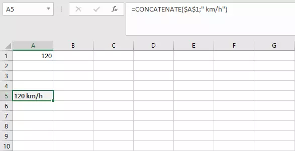
The value from cell A1 (in this case, the reference is absolute, so it does not change, even if the formula is shifted) is combined with a text. To prevent the word from running directly into the value, the text module begins with a space.

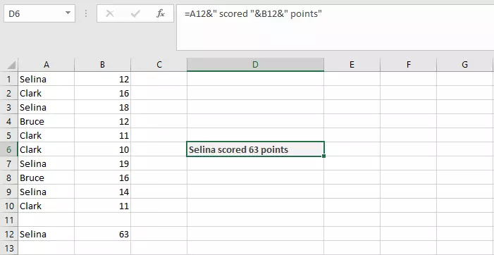
In this way, Excel allows you to write entire sentences. If you combine one or more cells with text, you can output complex content comprehensibly. Let’s assume we have a list of names and multiple point scores for each participant. We want to sum up the point scores by name. To do this, we can use the SUMIF function.

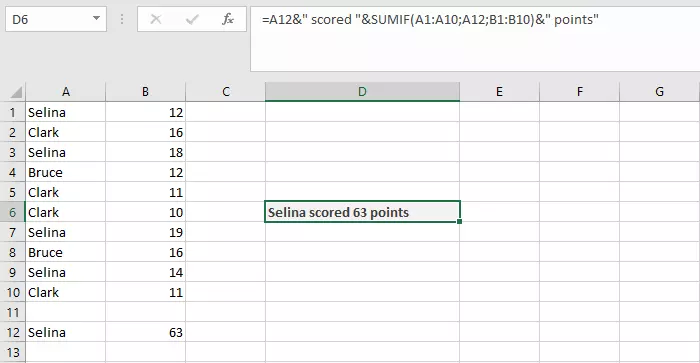
Excel now sums up all point scores corresponding to the name we entered in cell D2. You can also choose the name conveniently via a drop-down menu. Now we can combine the cells in a concatenation of the names and results.

Because the CONCATENATE function accepts additional functions as arguments, we don’t need auxiliary cells and can integrate the SUMIF function directly into the formula.

In Excel, CONCATENATE is combined frequently with the TEXT function. This function converts numerical values into text, in a specified format and adds corresponding symbols (e.g. for currencies). That makes is a valuable function in combination with concatenation.

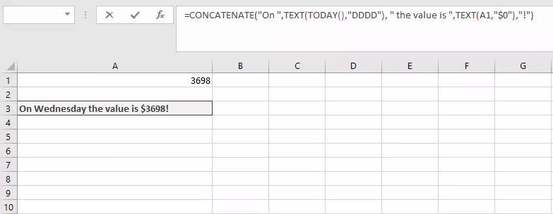
We can generate a complete phrase with this formula. The first TEXT function inserts the current day of the week, the second extracts a number from a cell and formats the value as a sum of money.

Since Excel 2019, Microsoft has introduced two new functions related to the CONCATENATE function. These expand on the options provided by Excel CONCATENATE and therefore are available separately. The 2019 version of Excel thus remains compatible with older Excel worksheets.

The CONCAT function works much like CONCATENATE. Just like the older version, it lets you combine various elements. One advantage over the older version is that you can enter entire ranges and do not need to fill a separate argument for every cell.

The contents from the various cells are inserted consecutively into the result text. The function proceeds row by row. That means that A1 is followed by B1, not A2. CONCAT doesn’t insert spaces automatically. If you want to separate individual contents from one another, you have to use the same procedure as in CONCATENATE.

The new TEXTJOIN function is different: While the aim is the same, the syntax is different. You can specify the separator you want to use directly in this function.

In TEXTJOIN, you first enter whether you want to use a delimiter (i.e. separator), and if so, which one. This could be either a space or a hyphen, for example. You have to enclose this entry in quotes. Then you indicate whether the function should include empty cells or not. To do so, enter TRUE or FALSE. Similar to other functions, the actual elements to be joined follow.

Just like CONCAT, you can also enter an entire cell range for TEXTJOIN. Thanks to the changed syntax, you can now insert separators between the individual elements.