How to use INDEX in Excel

Functions like VLOOKUP, INDIRECT, or MATCH allow you to work with data efficiently. With Excel INDEX, you can quickly and easily return the value of a cell.

Quick guide for Excel INDEX¶

1. Decide where Excel INDEX should be applied.
2. In two separate cells, specify values for row and column to determine the cell whose value you want to return.
3. In a third cell, specify the Excel INDEX function: =INDEX(Array; Row; Column).

What is the INDEX function in Excel used for?¶

With the help of Excel INDEX, you can reproduce the content of any cell in another cell. This is why the formula contains coordinates. Based on the column and row specified, the function determines the desired value from an area that is defined by the user. This can then be shown directly in another cell or used in another function.

Since the specification is done through columns and rows, the Excel INDEX function is also very useful when working with arrays. In an array, Excel can read out the corresponding value for two specified factors.

What is the syntax for Excel INDEX?¶

The function uses a clear syntax. The user enters the area to be searched as a parameter and then the coordinates of the desired cell.

=INDEX(array; row; column)

The following parameters are used in the function:

• Array, defined by the top-left and bottom-right cell
• Row, in which the desired cell is located
• Column, in which the desired cell is located

The array is always defined using two cells, separated by a colon. If it only contains a single column or a single row, you only need to include one additional parameter. The INDEX function in Excel will automatically understand whether you mean the corresponding row or column.

You can either enter the coordinates directly as a number or establish a cell reference. The numbers are then contained in the cells specified. The parameter always relates to the selected area and not to the worksheet, for example. So, if the array begins in cell C2, the D column is number 2 and not number 4.

Practical examples of how to use the Excel INDEX function¶

The simplest way to use the Excel INDEX function is to reproduce the content of a specific cell. Cell references can be used to make working with the formula a little easier. This way, you can enter the column and row parameters directly in a cell and dynamically adjust the formula.

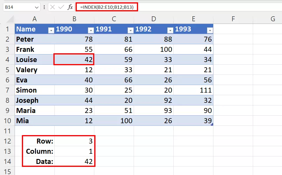
=INDEX(B2:E10;B12;B13)

We entered the column and row parameters in the cells B12 and B13. In this example, it’s important to note that the area within our Excel INDEX formula does not include the outer labels (name and birth year). Therefore, the correct result in our case is the first entry for Louise (‘42’), which is in line 3 column 1 of the specified range.

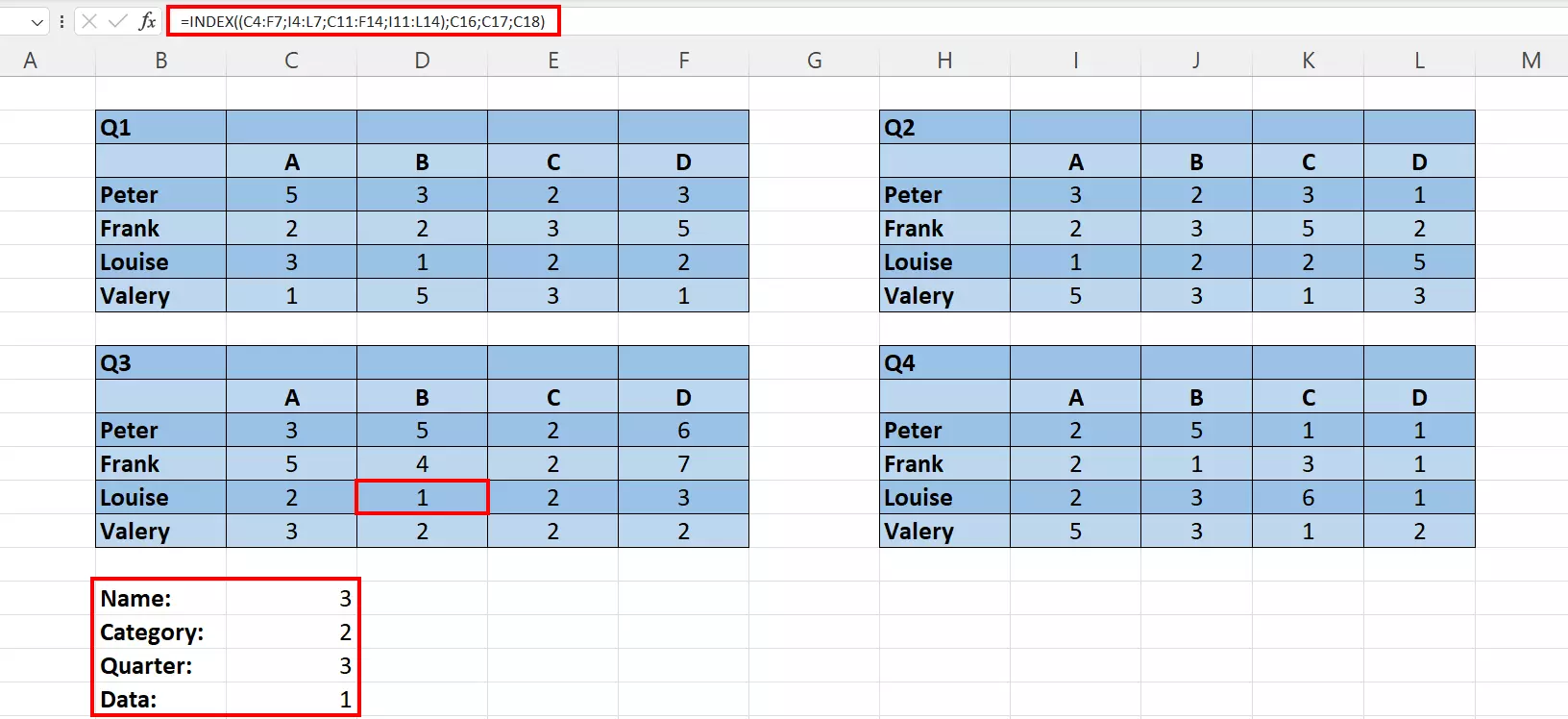
You can expand the formula if you have multiple tables with the same structure. Let’s assume we have four tables – one for every quarter. The structure of the tables is the same, meaning the columns and rows are laid out identically.

=INDEX((C4:F7;I4:L7;C11:F14;I11:L14);C16;C17;C18)

We have the parameters for rows, columns, and the area via cell references. To make it easier, you can also create Excel drop-down lists for the parameter selection. Excel will then create a helpful form for selecting the correct value with the Excel INDEX function.

How to combine Excel INDEX with other functions¶

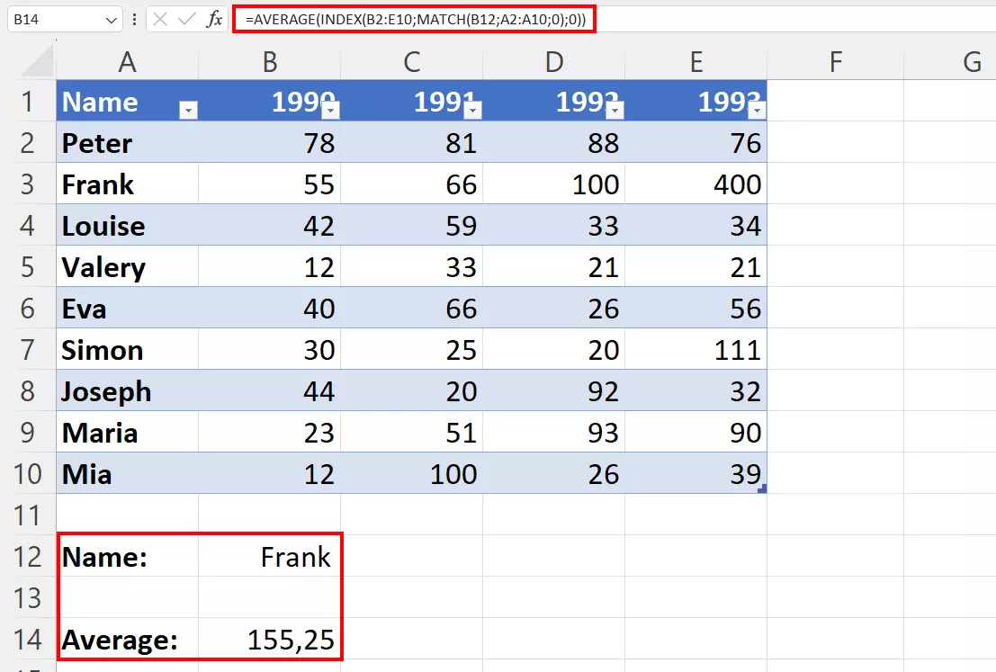
With Excel Index, you can also combine mathematical or statistical functions such as AVERAGE. In this case, INDEX (again in conjunction with MATCH) indicates the area for which the mean value is to be calculated. Rather than inserting it directly into the formula, you can dynamically change the selection area via the arrangement of the formula.

=AVERAGE(INDEX(B2:E10;MATCH(B12;A2:A10;0);0))

For the value in cell B12 (in the example: ‘Frank’), you get the respective mean value. This technique also works well when combined with the Excel SUM function.