How to use VLOOKUP in Excel

VLOOKUP makes working with Excel considerably easier. You can save yourself the trouble of searching through a large data collection manually and instead use the VLOOKUP formula to render results into another cell instantly. So that you can fully benefit from this Excel function, we’ll explain to you step by step how to do a VLOOKUP in Excel using a simple example as well as offer different ideas for how the function can be used.

What is VLOOKUP?

VLOOKUP is one of the most useful Excel features and belongs to the lookup and reference functions. Imagine you have a table consisting of several columns containing data that’s been collected, and you need the right result for a certain search query. We’ll use a member directory as an example:

You might know the name of a person but need to find their phone number. With the VLOOKUP formula you don’t need to search the entire spreadsheet for the name. The function searches a column of the directory from top to bottom until it finds the name you’re looking for. Then it returns the corresponding value from the column where the phone numbers are stored.

However, VLOOKUP is limited in that the function only returns one result — namely the first one. If two people in the directory have the same name, the function will only return the number of the first person. In addition, the search criterion must always be in the column furthest to the left. As a result, the table must be structured in such a way that no relevant columns appear to the left of the column where the search is being performed.

What is the syntax for VLOOKUP?

To accurately use VLOOKUP in Excel, you need to know how to enter the formula correctly. Every Excel function has a specific syntax that must be entered exactly as it is, otherwise the command will not return the correct result, or an error message will be displayed. The VLOOKUP syntax is as follows:

=VLOOKUP(lookup_value; table_array; col_index_num; range_lookup)

Now, let’s take a closer look at the different parameters:

• lookup_value: This refers to the value that you are looking for. You can enter the criterion directly into the formula in words using quotation marks or enter the specific cell that contains the data.
• table_array: This is the second argument, or piece of information required, when inserting the VLOOKUP formula. This argument refers to a group of cells that contain the source data and where you will be returning values from.
• col_index_num: This refers to the location of the column within the specified table location in numeric value. Note: Column D does not automatically have the index number 4. If you start the data area from column B, then D would have the column index number 3.
• range_lookup: Should the results be exact or just approximately equal? With a 0 or FALSE only the exact match will be shown. 1 or TRUE will allow for other input and then return the next smallest value. The entry of this parameter is optional. If you leave this part blank, it will take the 1 function by default.

Here’s an example of how the VLOOKUP function in Excel looks:

=VLOOKUP("Turn";B1:D50;2;FALSE)

VLOOKUP example

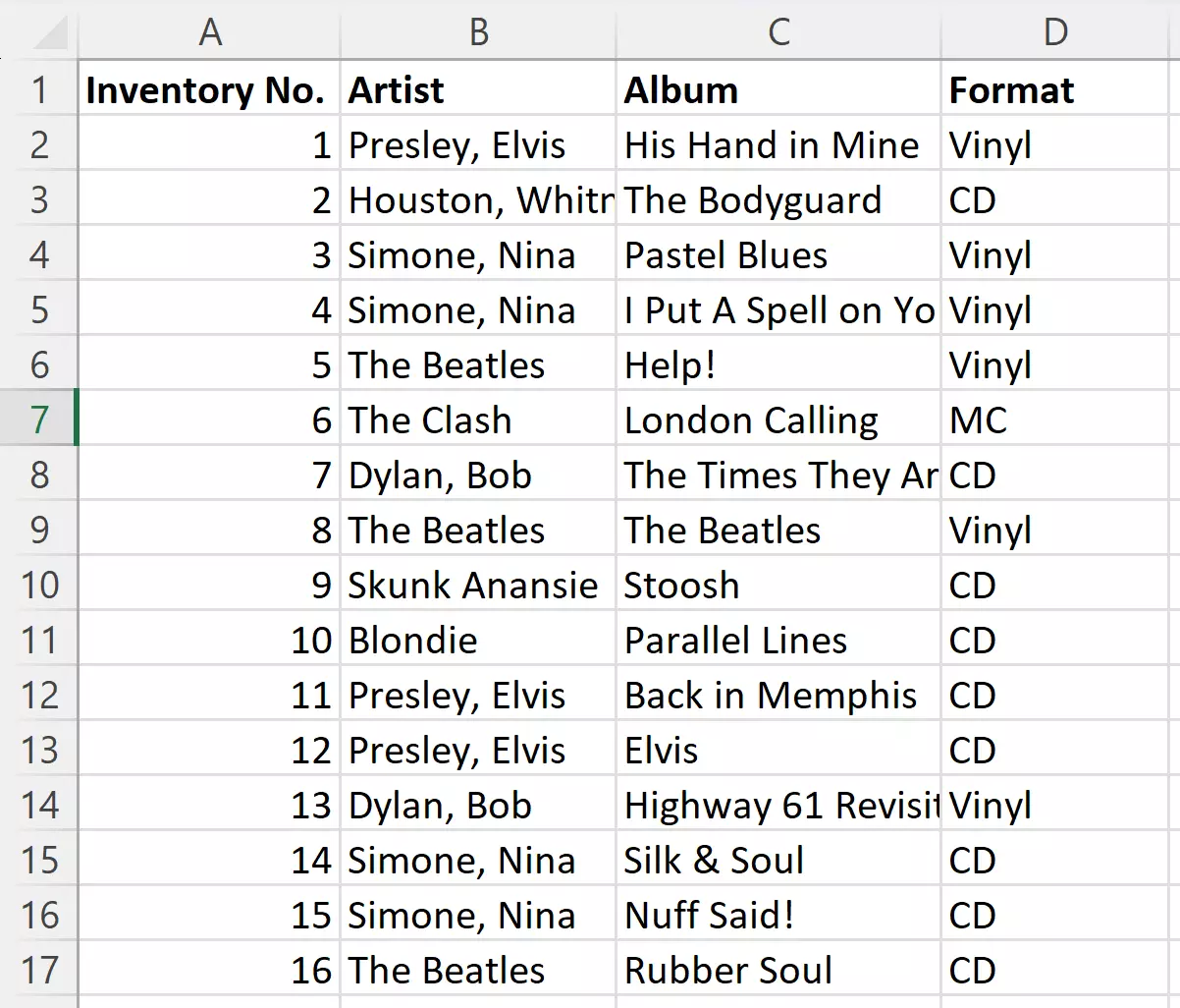
So how do you use VLOOKUP exactly? The function is particularly useful when it comes to searching large collections of data and delivering a specific result. As an example, let’s imagine we have a music collection and create a directory in Excel. Every album is given its own entry, although it is not sorted by name but simply by when it was added to the collection.

Find values with VLOOKUP

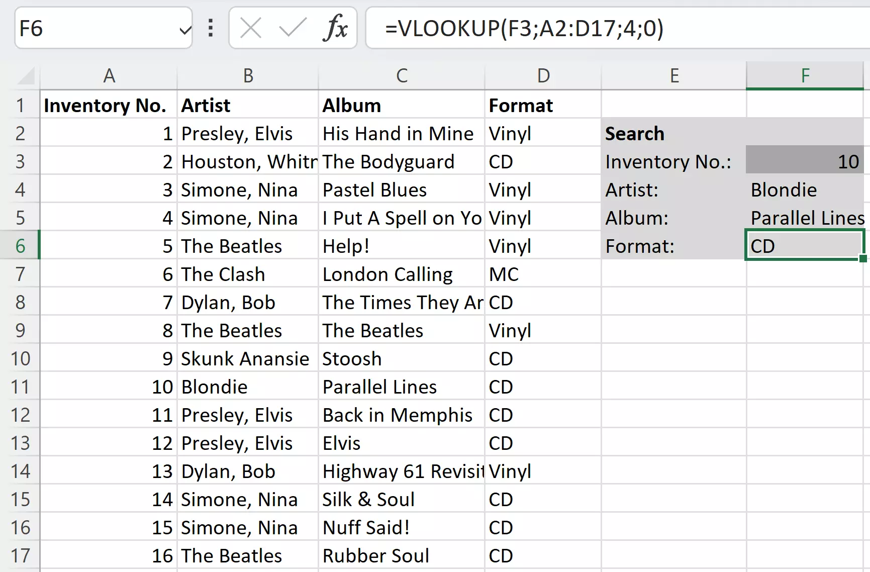
We want to find out which album is in inventory spot number 10. To do this, we can use the VLOOKUP function in Excel:

=VLOOKUP(10;A2:D17;3;0)

The cell in which we entered the function should now display ‘Parallel Lines’.

What if you want to carry out this search more than once? It is possible to merge VLOOKUP into a form that is also connected to the artists and format. For this, we don’t add the lookup value (the inventory number in our example) directly into the formula, but instead reference the cell where we want the result to be displayed:

=VLOOKUP(G2;A2:D17;3;0)

We put the same function in two more cells but change the column index number to 2 and 4.

Combine VLOOKUP with other functions

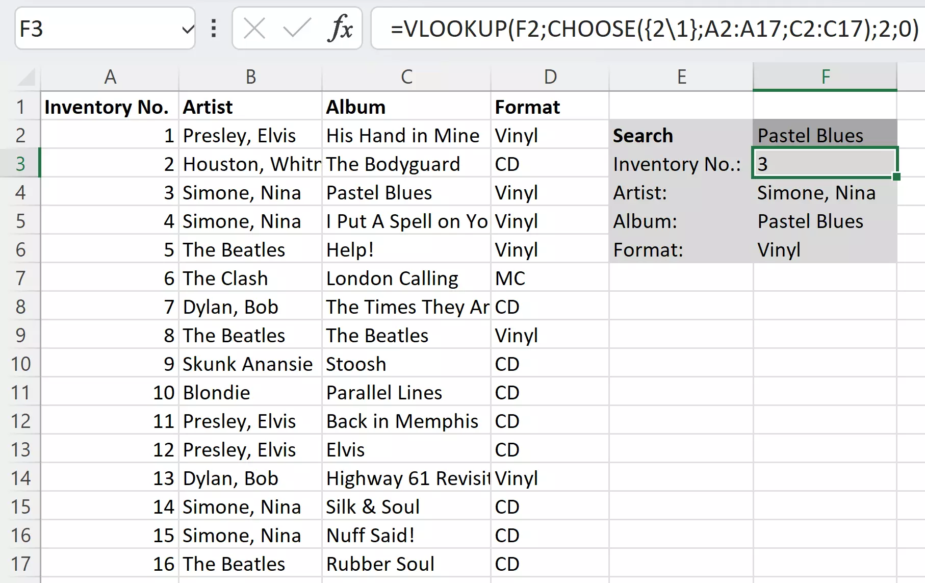
Now, in most cases, the situation is the complete opposite of what we’ve shown in the examples above. You know which album you are looking for and would like to find the inventory number or artist. Using the CHOOSE function, you can get VLOOKUP to do this. This function allows you to essentially change the table location. It does this by displaying VLOOKUP columns in a different place than where they actually are. In the CHOOSE function, you can specify different areas and the order that they should be interpreted in:

= CHOOSE(Index;Value1;Value2;…)

For the value parameter, we use the columns from our table and then specify a reverse order in the index. The index tells the function the order in which it should interpret the columns. The index specification is done in curly brackets and the individual numbers are separated by dots. CHOOSE replaces the table location parameter in our example:

= LOOKUP(F2;CHOOSE({2.1};A2:A17;C2:C17);2;0)

Now the function for an album title gives us the appropriate inventory number. It is also possible to expand the values in CHOOSE and record the complete data area. In our example, this is not necessary. We can use the inventory number to determine the other values using simple VLOOKUP functions.