Google Sheets: conditional formatting explained

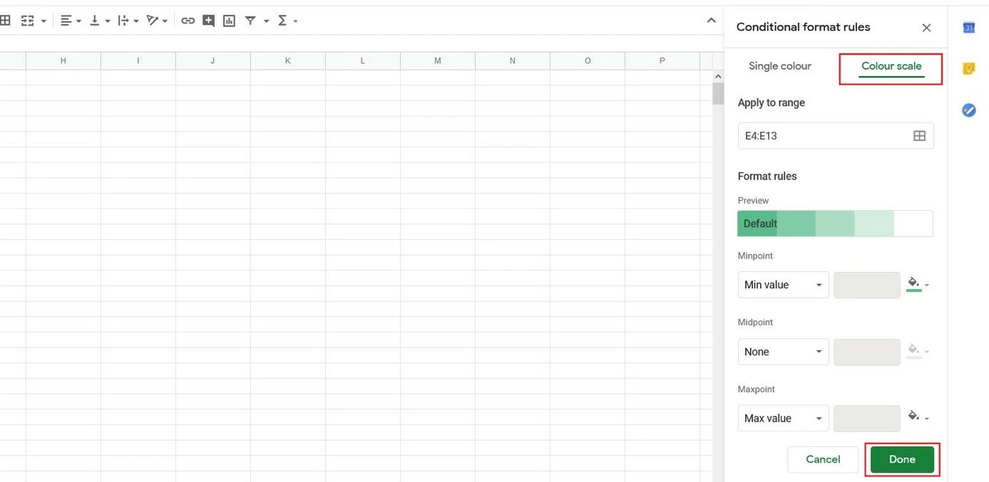
The simplest way to highlight specific information is to compare and relate individual entries to each other. Formatting options such as “Colour scale,” for example, are useful to highlight high values in a darker colour than lower values. Google automatically suggests a scale of green tones, but users can choose their own colours. To format highlighting options in your Google Sheets project, follow these steps:

1. Mark the desired range of values.
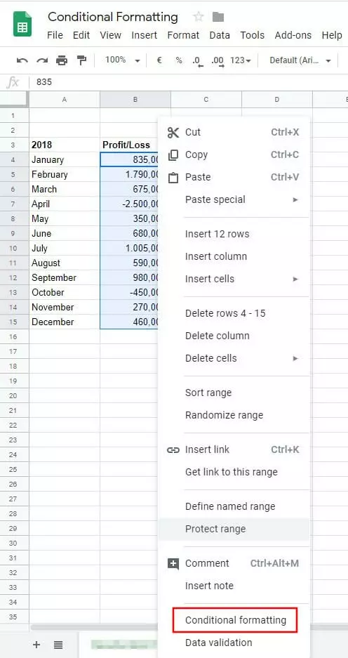
2. Right-click on the selected area and choose “Conditional formatting.”
3. In the lower right side menu, select “Colour scale.” You can now choose to continue with the green colour scale or select your preferred colour. Click on “Done” when you’re finished.

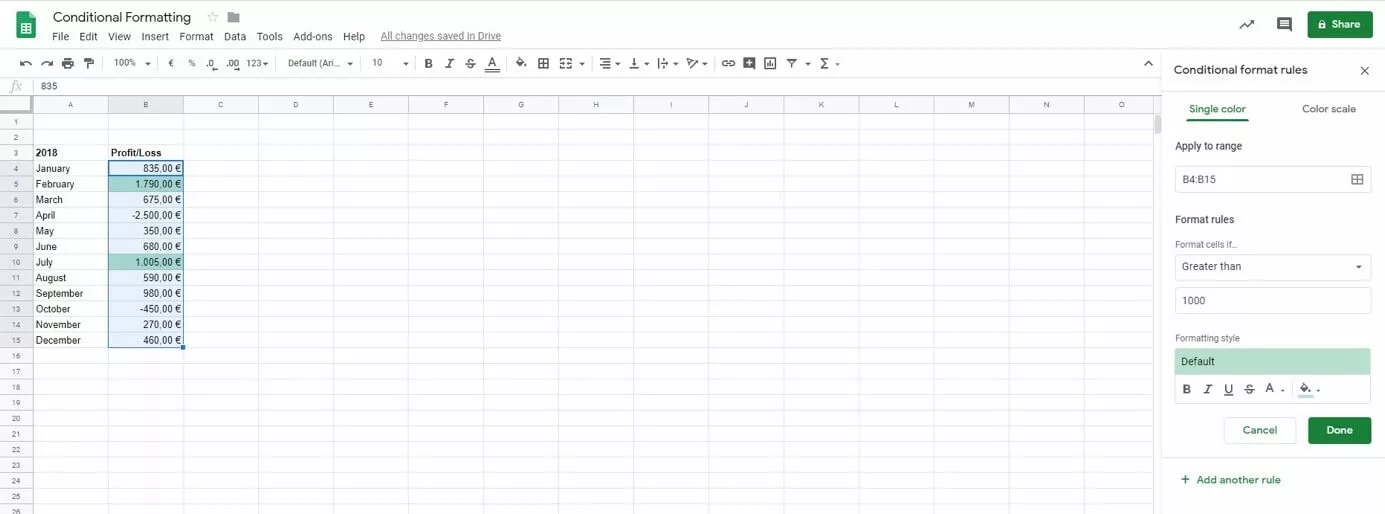
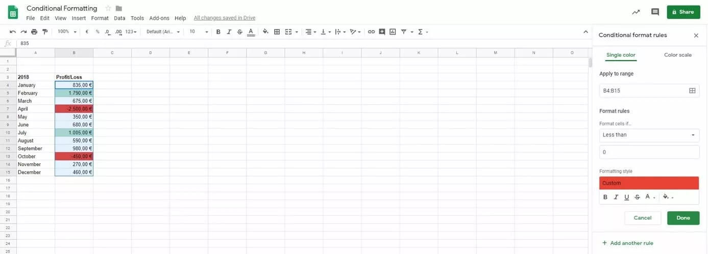
If you’re working with an extensive profit-loss table and need an overview of the months during which the business performed particularly well, conditional formatting can be defined based on rules and exact values. The following example is based on a table of revenue and outgoings over a period of 12 months. Here, we want to highlight cells that meet the following conditions: profits over $1,000 are to be automatically highlighted in green, and losses will be shown in red.

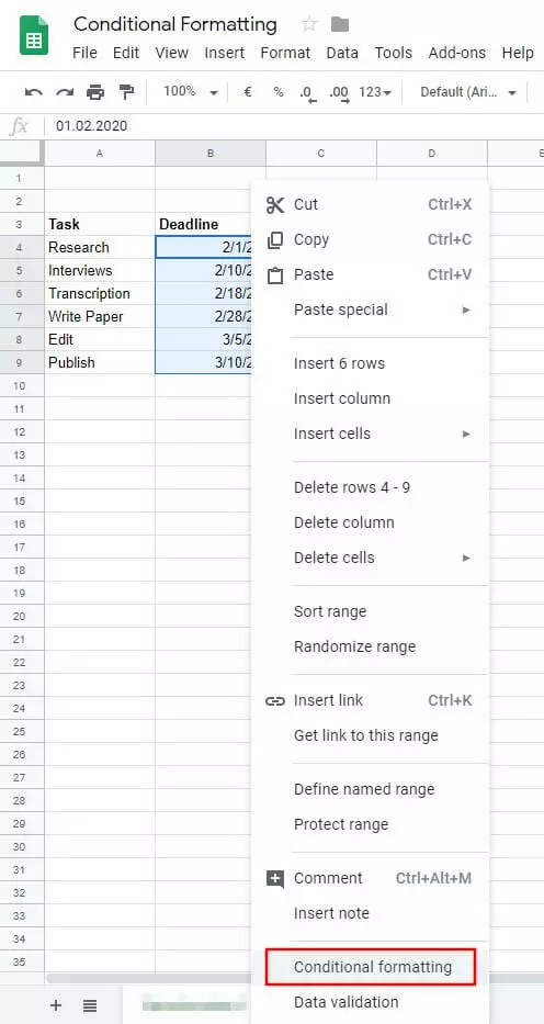
1. Mark the range of values in the spreadsheet you want to apply the conditions to. Right-click anywhere in the selection and select “Conditional formatting.”

2. The dialogue window “Conditional format rules” will open up in which conditions and formatting can be further defined. Select “Format cells if…” from the drop-down menu and choose “Greater than.” In the field below, enter the value “1000.” All values within the selected range that are greater than 1,000 will be automatically highlighted in green.

3. By selecting “Add another rule,” you can specify additional conditions. In this example, we’re trying to highlight all cells with values smaller than “0” in red signifying losses. Add another rule and choose “Smaller than” and enter “0.” Change the formatting colour to red. Hit “Done” when you’re ready.

Aside from conditional formatting via defined rules for values, text, and dates, you can also specify your own formulas to format data. A user-defined formula allows you to highlight cells which meet the conditions of your formula. This could be useful to highlight future dates, for example, as shown in this example:

1. Mark the range of values in the spreadsheet you want to apply the conditions to. Right-click anywhere in the selection and select “Conditional formatting.”

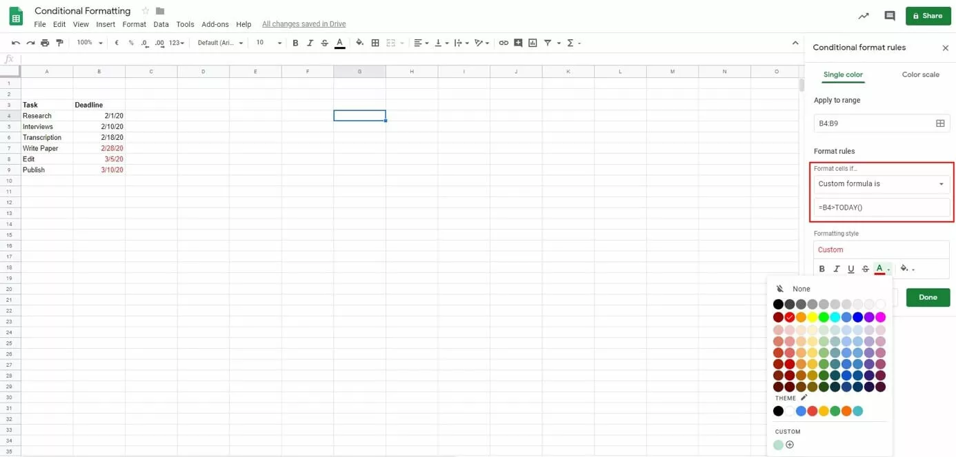
2. In the settings window “Conditional format rules” select “Format cells if” and choose “Custom formula is” from the drop-down menu. Enter the desired formula. In this example, the formula is “=B4>TODAY()”. Then select your preferred formatting. In the example below, all future dates will be marked in red.

3. Confirm your conditional formatting by clicking on “Done.” If you right-click into one of the conditionally formatted cells and click on the “Conditional format rules,” you can see the active formatting in the selected cell. If necessary, you can also add another rule.