Excel: conditional formatting – what is it?
Since Microsoft 2007, Excel, the popular spreadsheet processing software, has included conditional formatting. This type of formatting lets you visualise large and complex data sets, allowing you to spot data trends and missing data more easily and quickly. The cells to be distinguished depend on pre-specified fixed conditions. The advantage of conditional formatting which is used across a range of different Office programs is that only cells fulfilling certain criteria are highlighted or otherwise visually represented.
- Free website protection with SSL Wildcard included
- Free private registration for greater privacy
- Free Domain Connect for easy DNS setup
Conditional formatting: popular areas of application
There are three main areas of application for using conditional formatting in Excel:
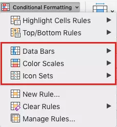
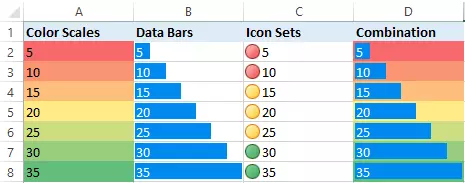
- Visualisation of values: All numbers in a defined cell range are considered in relation to one another. With this type of conditional formatting, the appearance of the cells is based on the size of the values. If values are negative, larger, or smaller than the other numbers, they are highlighted.
- Checking data: Depending on data volume, assessing each individual cell for deviations is a time-consuming process. That’s where conditional formatting can be useful. By defining certain conditions, only those cells are highlighted that you are looking for.
- Filter double and distinct values: If you are looking to create a list of distinct values, you can use conditional formatting formulas in Excel and co. You can filter defined values by masking double values. Alternatively, you could also delete duplicate values.
Excel: conditional formatting based on values
Conditional Excel formatting is also useful when comparing a list of different values. In just a few clicks, you can compare individual values with one another. A defined cell range can be analysed and visualised with colours. For example, maximum values are marked in green, whilst minimum values are highlighted in red. Alternatively, data beams or symbols like darts can be used to represent predefined data and results.
Earlier versions of Excel do not include multiple options for conditional formatting such as data bars or symbols. To make use of the latest features in Excel, you should use the latest version of the spreadsheet software. Excel is available as part of the IONOS Microsoft 365 Business package, which also includes Word, PowerPoint, etc. and a personal domain.
Conditional formatting based on rules
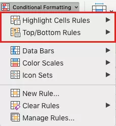
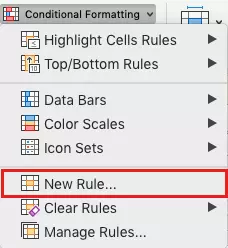
Specifying conditional formatting based on defined rules makes it a little more flexible. Because this type of formatting is based on threshold values, only certain cell divisions are considered. Depending on your needs, you can format defined or upper/lower values. This includes predefined formatting rules for the top 10 upper/lower or 10% of elements. By clicking on “Highlight Cells Rules,” you can also choose between:
- Larger than…
- Smaller than…
- Between…
- Equal to…
- Text…
- Date…
- Double values…
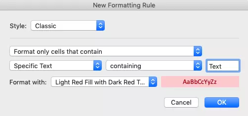
If instead of working with numbers you tend to work with text entries and want to highlight cells containing certain terms, click on “Highlight Cells Rules” > “Text” and enter the text you want to filter by. Click “OK” and the information will be highlighted.
- Up to 50 GB Exchange email account
- Outlook Web App and collaboration tools
- Expert support & setup service
Conditional formatting using formulas
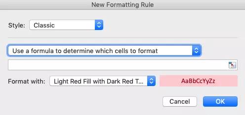
For even more flexibility using conditional formatting, Excel users can apply individual formulas. Instead of relying on predefined Excel formulas, you can specify their own rules. This allows for unlimited possibilities when it comes to checking your data. The right formula can, for example, be used to compare a range of numbers to a reference table, as shown in this YouTube video.
 To display this video, third-party cookies are required. You can access and change your cookie settings here.
 User examples for conditional formatting in Excel
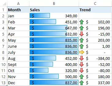
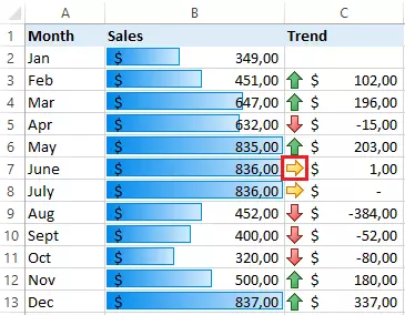
In order to add the data bars in column B, select cells B2 to B13 and click on the following:
- “Conditional formatting”
- “Data bars”
- “Fill with…” (make a selection)
Now, select cells C3 to C13 and click on:
- “Conditional formatting”
- “Icon Sets”
- “Directions”
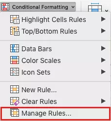
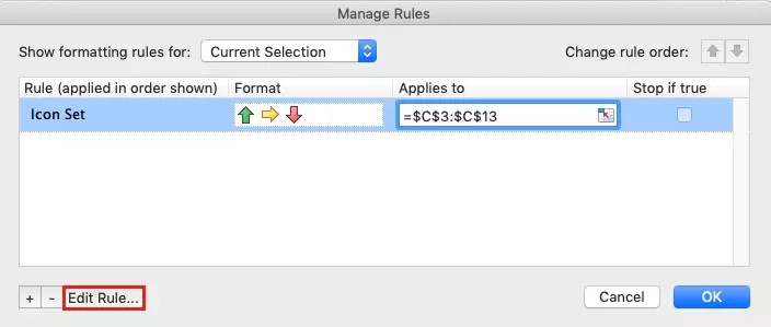
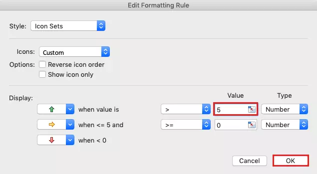
If, for example, you want to show an upward trend in column C only when profits increase by at least €5 compared to the previous month, the rules need to be edited. Mark cells C3 to C13 and click on “Conditional formatting.” Select “Manage Rules…” and “Edit Rules.”
The dialogue for the conditional formatting manager will pop up again. Click “OK” to confirm your chosen changes for the selected cell range. The upward trend (green arrow) in cell C7 will no longer be shown because the profit increase of at least $5 was not achieved from May to June.
The above is a simple example illustrating the possibilities of using Excel’s “Conditional Formatting” feature. Generally, the more confident you are using Excel formulas and functions, the more effectively and flexibly you will be able to use these features.
- Familiar Google tools all in one place
- Using Gmail with your domain from IONOS
- Configure business Gmail for your domain


