

Time recording in Excel: How to create a timesheet

More and more companies are introducing flexible working hours in their business. This has clear advantages for productivity and employee satisfaction, but also requires a certain level of trust. A system for recording working time is usually used for this purpose. This serves as proof of how much the employee has worked and the boss can then use it for quality control and weekly or monthly accounting. All you need for an electronic timesheet is the Excel spreadsheet software - and our step-by-step instructions.
- Up to 50 GB Exchange email account
- Outlook Web App and collaboration tools
- Expert support & setup service
Requirements for a professional timesheet
What makes a professional timesheet in Excel so special? Employees, employers, and lawmakers have quite different demands.
Requirements from the employee’s point of view
From the employee's point of view, a time recording system must be easy to use. After all, regularly having to document your own working times and break times means additional effort and interruptions to your workflow. The structure and design of an Excel timesheet must therefore make it immediately clear which information is relevant and where and how the corresponding data must be entered. A clear structure, helpful colour scheme, and limiting everything to the essentials can help a lot. Basically, the easier you make it for your employees, the more likely it is that the time recording will be regularly filled out, delivered on time, and be correct.
Requirements from the employer’s point of view
Since recording working time is relevant for checking employee performance as well as for payroll accounting, there are often some complex calculations to be done. Ideally, the Excel spreadsheet should do these calculations automatically in order to save employees and employers time and effort. Corresponding functions can be integrated into the file and will reduce the amount of errors for regular time recording in the future.
Requirements from a legal point of view
Under the UK Working Time Regulations, employers have to keep records to show that the weekly working time limit is being adhered to. Employees aren’t allowed by law to work more than 48-hour weeks unless they have opted-out, which means they can work as many hours as they like. Those who have not opted out can still work more than 48 hours a week as long as the average number of hours per week doesn’t exceed 48 hours.
The timesheets can also be used to prove that night workers aren’t working more than 8 hours in any 24 hour shift, which isn’t allowed. Young workers also aren’t permitted to work over 8 hours a day, or more than 40 hours in a week.
The employer must keep records for two years from the date they were made. Failure to comply can result in an unlimited fine.
Step-by-step instructions: Creating timesheets in Excel
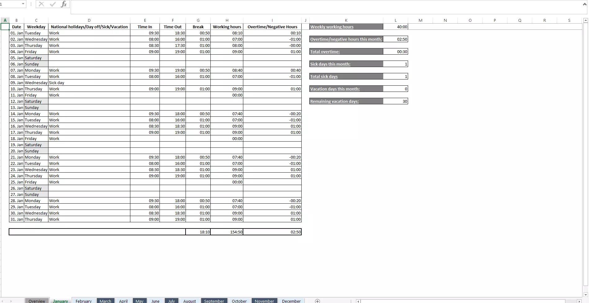
The following example shows a timesheet for time recording in Excel. It serves as proof of how many hours an employee has worked.
For this, the employee can enter the times when they started the shift or finished it. They also enter the beginning and end time of their breaks. The formulas in the Excel spreadsheet automatically calculate how many hours were worked, and at the same time determine any accumulated plus and minus hours. This saves the employer a lot of time and effort during payroll accounting. The employee also has the option of being compensated for holiday days and sick days, which are automatically recorded. Clear formatting and colour design should clearly emphasise the most important information (the actual working hours and plus/minus hours).

The Excel timesheet template from IONOS can be downloaded free of charge from the following link and used straightaway:
In the following step-by-step instructions, we explain the individual steps required to create the timesheet template.
Step 1: Setting up headers and columns
Here is how you equip the header of the Excel spreadsheet with all the necessary information, set up the columns, and format your timesheet clearly:
- In cell A1, enter the name of the employee.
- In cell D1, enter the daily target working time of the employee using the format hh:mm (h = hours, m = minutes), for example, 08:00 (8 a.m.). This value serves as a reference for the calculation formulas that we plan to include later in the table.
- A small aid to help your employees: a current date display, which makes it easier for them to find the right row in the time sheet. To do this, enter the formula =TODAY() in cell H1 and confirm by clicking on “enter”.
- Another aid: In row 2 you can explain which email address (e.g. the HR department), the timesheet should be sent to and which subject the email should have.
- In row 3, enter the column headings “Date”, “Time in”, “Start of break”, “End of break”, “Time out”, “Absences”, “Actual working hours” and “Plus/minus hours” one after the other.
- Format your table as you like. Use bold writing and different fonts, sizes and colours as you see fit. Keep the column widths consistent to create a better overview and be more visually appealing. Connected cells and different fill colours can help to separate individual areas from each other. The “Transfer format” button in the upper left corner of the menu helps you to speed up the design process.
- Finally, freeze the upper three rows of your table so that they remain visible to the employee even when they scroll down. To do this, select cell A4. Now click on the “Freeze panes” button under the “View” tab and select “Freeze panes”. Now all rows above cell A4 are fixed in place.
You can also copy all formulas listed in this article directly into your Excel spreadsheet. However, do not forget to press the Enter key after each insertion or input so that the formula is saved correctly.
Step 2: Insert continuous date
Here’s how to add a continuous date to your Excel timesheet and highlight the weekends in colour:
- In cell A4, enter the first date that you want to start recording the working time.
- Under the “Home” tab in the “Number” area, click the small arrow next to “Date” and select the “Long Date” format. The date is now displayed in long form and includes the day of the week.
- Click on the small square in the lower right corner of the selected cell A4 and hold down the mouse button. Now drag the arrow downwards until the area covers a full seven-day week.
- Select all columns. Click on column A, hold down the mouse button and drag all the way to column H.
- Click on “Home”, then in the “Styles” section, you should see “Conditional Formatting”. Click on this.
- Click on “New Rule...” in the following menu. A separate window will open.
- Under “Select a Rule Type:”, click “Use a formula to determine which cells to format”.
- Under “Format values where this formula is true,” copy the following calculation to the dialogue box: =WEEKDAY($A1;2)>=6 (this formula means in plain language: “The following applies to all Saturdays and Sundays in column A”).
- Click on the “Format...” button. Another window will open.
- In the “Fill” tab, select any colour for marking the weekends and click “OK”. Confirm the entry again with “OK”. All Saturdays and Sundays should now be highlighted in colour.
Don’t worry: You only need to set up this complicated formatting, rules and formulas just the one time. To add more cells with the same properties, simply click on the small square in the lower right corner of your cell and drag it down.
Step 3: Configuring absence options
How to add a drop-down menu to the absences column of your timesheet table:
- In column F (“Absences”), select the first cell that belongs to a weekday. In our case this is F5.
- Select the “Data” tab in the horizontal menu.
- Click the “Data Verification” button in the Data Tools section. A new window will open.
- Select in the “Settings” tab, the “List” option, which can be found under “Validation criteria” > “Allow”.
- Remove the tick for “Ignore blank”.
- In the “Source” dialog box, type the options you want to be available in the drop-down menu. Remember to separate the options with a semicolon. In our example it looks like this: Holiday;Illness;Mobile Office.
- Confirm your entry with “OK”.
- The cell in column F now has a drop-down menu added. To add it to the other days of the week, simply copy it using [Ctrl] + [C] / [Ctrl] + [V]. Alternatively, you can use the small square in the lower right corner of the cell, which is a faster way.
If an employee wants to undo their selection in the drop-down menu, all they have to do is press the [Del] key.
Step 4: Calculate actual working hours
This is how you can get Excel to automatically calculate the actual working hours of your employees:
- Select column G (“Actual working hours”).
- Under “Home” > “Number” click on the small arrow next to “Number” in the box and select “More...” at the end of the drop-down menu. A new window will open.
- Under “Category”, select “Custom” and enter the following formatting in the dialog box under “Type”: [hh]:mm (this commands Excel to include the absolute number of hours in the total instead of always starting from zero after 12:00).
- Confirm the entry with “OK”.
- Copy the following formula into the first cell in column G that belongs to a weekday (in our case this is G5): =IF(OR(F5="Holiday";F5="Illness");$D$1;E5-(D5-C5)-B5).
This rather complicated looking if-then formula tells Excel the following: “If in column F (“Absences”), “Holiday” or “Illness” is entered instead of a date, the 8 target daily hours from cell D1 should be recorded as actual working hours (if “Mobile Office” is entered, nothing should happen). If, on the other hand, column F remains empty, the working hours should be calculated regularly according to the following formula: E5 (time out) - (D5 (end of break) - C5 (start of break)) - B5 (time in)." As usual, you can apply this formula to all other days of the week using the small square. The formula $D$1 ensures that the same target daily hours are always used as a reference.
Now the actual working hours have to be added to the number of weekly hours:
- In column G, in the first cell that belongs to a Saturday (for us this is G10), enter the following formula: =SUM(G5:G9).
- Alternatively, you can click on the “AutoSum” button in the “Formulas” tab and select the “Sum” option. Excel then automatically determines the correct formula.
Step 5: Calculate plus/minus hours
Here’s how to get Excel to calculate both plus and minus hours for an employee:
- Format the column H (“plus/minus hours”) as [hh]:mm - use the same procedure as for column G (“actual working hours”).
- Since Excel cannot display negative times by default, you have to make a small detour to “Options”. Click on “Advanced” and search for “When calculating this workbook:”. Set a tick in front of “Use 1904 date system”. Confirm the entry by clicking on “OK”.
- In our example, we now enter the following formula in cell H5: =G5-$D$1 (this tells Excel to settle the actual working hours with the target working hours).
- Transfer the formula to all other weekdays as usual.
- To total the plus/minus hours, you can use the “AutoSum” function again or enter the formula =SUM(H5:H9) manually.
Overview of all necessary formulas
In the following section, we have summarised all the practical formulas that you need for Excel time recording. If you copy our example directly, you can adopt these formulas without needing to make any changes. If, on the other hand, you want to create your own timesheet design, you must adjust the cell specifications accordingly. Please refer to the screenshot above and our downloadable template.
| Purpose | Formula (in relation to our example) |
|---|---|
| Current date | =TODAY() |
| Highlight weekends in colour | =WEEKDAY($A1;2)>=6 |
| Daily actual working hours | =IF(OR(F5="Holiday";F5="Illness");$D$1;E5-(D5-C5)-B5) |
| Total target working hours | =SUM(G5:G9) |
| Daily plus/minus hours | =G5-$D$1 |
| Total plus/minus hours | =SUM(H5:H9) |
Excel time recording in use
Lastly, we’ll explain how to reuse your completed Excel time recording template, equip it with partial write protection, and send it to your employees.
Reusing the Excel template
You’ve now got yourself a professional Excel timesheet template that currently only covers a single week. To extend it to any amount of time, apply this trick again: Select the entire week including all columns with the mouse, click and hold the small square in the lower right corner of the selected area and drag it downwards. As you can see, Excel automatically detects a recurring pattern and replicates all formatting, drop-down menus, formulas, and rules for all continuous data. This allows you to reuse your template over and over again.
Equip Excel timesheet template with partial write protection
Your employee enters the times that they start work and when their breaks begin, as well as when they finish work and what time their breaks end in columns B, C, D, E using the hh:mm format (e.g. 08:30). They enter holiday and sick days in column F. Apart from this, they don’t need to make changes to the contents and structure of the timesheet. For this purpose, it makes sense to equip the Excel table with a partial write protection.
This is how to do it:
- If the active Excel worksheet is “locked”, cells can’t be edited. To implement only partial write protection, you must first change this setting.
- To do this, select the entire table by clicking on the point of intersection between the columns and rows (top left).
- Now click on the small arrow in the lower right corner of the “Alignment” area under the “Home” tab to open the “Format Cells” dialogue box. You can also use the key combination [Ctrl] + [1].
- Select the “Protection” tab and untick the “Locked” tick box.
- Confirm the entry with “OK”.
- Hold down the [Ctrl] key and use the mouse to select all the cells you want to protect. We recommend rows 1, 2 and 3 as well as column A.
- Return to the window with the “Locked” option and add the tick again.
Unfortunately, this method does not include the formulas in the G and H columns. To include them, proceed as follows:
- Press the key combination [Ctrl] + [G] to call up the “Go to” dialogue box.
- Click on the “Special...” button.
- Check “Formulas” and confirm with “OK”. Excel will now select all cells that contain formulas.
- Proceed as described in the previous tutorial to set all formulas to “Locked”.
Before you send the timesheet to your employees, you must activate the write protection:
- Click on the “Protect sheet” button in the “Review” tab.
- Under “Allow all users of this worksheet to:” remove the tick for “Select locked cells”.
- It’s also possible to set a password to protect the worksheet.
- Click “OK” (if you have entered a password, you will need to confirm it again).
Send Excel timesheet to employees
Save your timesheet in regular Excel format and send it to your employees by email. Remember to include instructions that explain the procedure for recording working times in an understandable way. Clarify, for example, which email address the completed timesheet should be sent to, and when. By specifying a fixed format for naming the Excel files (e.g. first name, last name, calendar week), it’s easy to assign the timesheets to the relevant employee later.
Some Excel alternatives also have functions for creating electronic timesheets
Reviewer

Anne-Laure Wolber
Anne-Laure has been part of the IONOS Digital Guide since its inception in 2016. As an expert in the startup category, she focuses primarily on the strategic integration of SEO, GEO and conversion rate optimisation. Over the years, she has also gained extensive experience in related performance disciplines such as lead generation and native advertising. As a polyglot, she leverages her multilingual background to develop content strategies with precision and impact for international audiences.